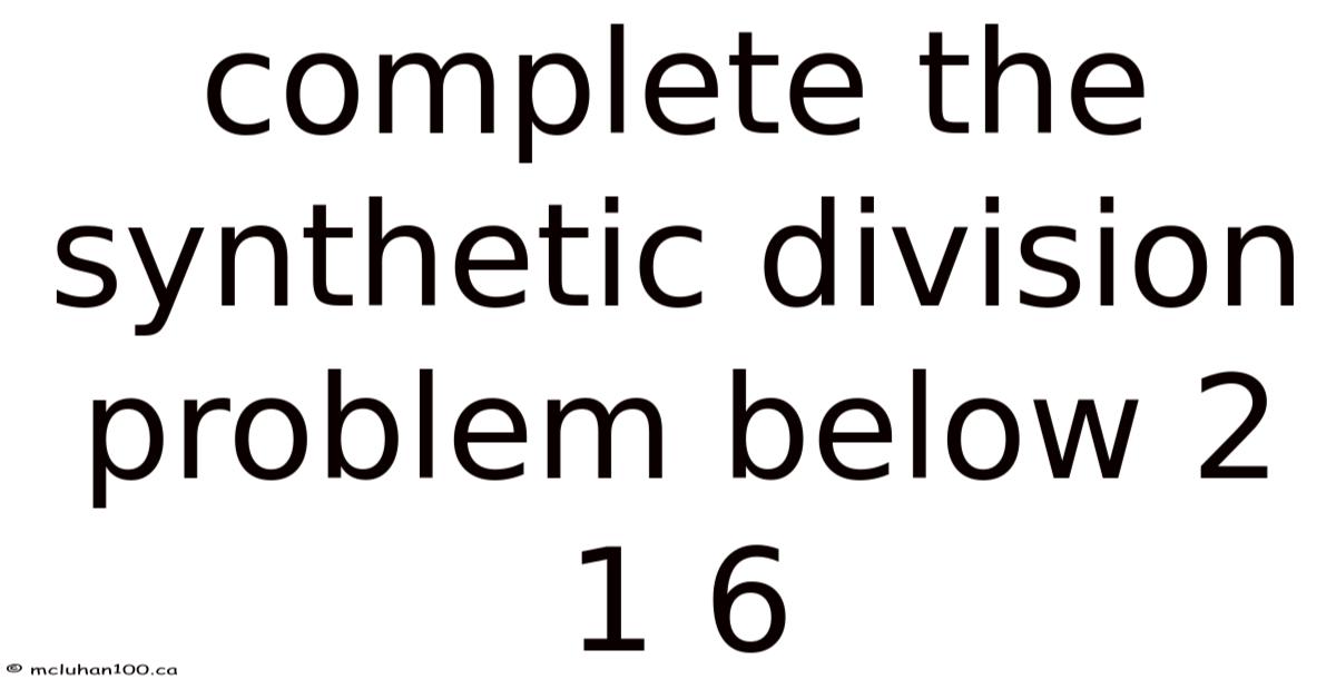
You're staring at a synthetic division setup — 2 | 1 6 — and your brain freezes. But the steps? Six. Day to day, been there. But one. Two. Day to day, the numbers look simple enough. They slip away right when you need them.
Here's the short version: you're dividing x + 6 by x − 2. That's why the answer is 1 with a remainder of 8. But if you only memorize the answer, you'll blank on the next one. Let's walk through it slow enough that the logic sticks.
What Is Synthetic Division
Synthetic division is a shortcut for dividing polynomials — but only when the divisor is linear, meaning it looks like x − c. In real terms, no fractions. No x² in the denominator. Just x minus a number Simple, but easy to overlook..
It replaces long division's messy columns with a clean, compact grid. You add. You write the coefficients. Repeat. You multiply. You bring one down. Done.
The catch? If you're dividing by x² + 3x + 2, synthetic division won't help. It only works for divisors of the form x − c. Long division or factoring is your path there.
Why the "c" matters
In x − c, the c is the number you put in the little box on the left. Which means that sign flip trips up more students than anything else. Consider this: read c. For x + 5, c = −5. In real terms, write the divisor as x − c. For x − 2, c = 2. Put that in the box Nothing fancy..
Why It Matters / Why People Care
You'll see synthetic division in algebra, precalculus, calculus, and even differential equations. It's how you:
- Find roots of polynomials fast
- Factor higher-degree polynomials after guessing one root
- Evaluate polynomials at specific values (Remainder Theorem)
- Simplify rational expressions before integrating
Here's the thing about the Remainder Theorem is the secret weapon here. That means synthetic division is function evaluation in disguise. On the flip side, when you divide f(x) by x − c, the remainder equals f(c). You're not just dividing — you're checking if c is a root, and finding f(c) at the same time.
In practice, this saves enormous time. Factoring a cubic? Day to day, guess a root, synthetic divide, get a quadratic, factor that. Done in thirty seconds instead of five minutes of long division Not complicated — just consistent. But it adds up..
How It Works (Step by Step)
Let's solve your exact problem: 2 | 1 6
Set up the grid
Draw an L-shape. Put the c-value (2) in the left corner. Write the coefficients of the dividend across the top — including zeros for any missing degrees.
Your dividend is x + 6. That's 1x¹ + 6x⁰. Coefficients: 1, 6. No missing terms, so no zeros needed Small thing, real impact..
2 | 1   6
  |_______
Bring down the first coefficient
Drop the 1 straight down below the line. This becomes the first coefficient of your quotient.
2 | 1   6
  |_______
    1
Multiply and add — the loop
Multiply the number you just brought down (1) by the c-value (2). Write the result (2) under the next coefficient (6) Which is the point..
2 | 1   6
  |    2
  |_______
    1
Add the column: 6 + 2 = 8. Write 8 below the line Easy to understand, harder to ignore..
2 | 1   6
  |    2
  |_______
    1   8
Read the answer
The numbers below the line are your quotient coefficients — but the degree drops by one. In practice, your dividend was degree 1 (x¹). Your quotient is degree 0 (a constant).
So the quotient is 1. The last number (8) is the remainder.
Result: (x + 6) ÷ (x − 2) = 1 + 8/(x − 2)
Or: x + 6 = (x − 2)(1) + 8
Check: (x − 2)(1) + 8 = x − 2 + 8 = x + 6. ✓
Another example — cubic divided by linear
Let's do 3 | 1 −2 −5 6 (that's x³ − 2x² − 5x + 6 divided by x − 3)
3 | 1   -2   -5   6
  |     3    3  -6
  |_______________
    1    1   -2   0
Quotient: 1x² + 1x − 2 = x² + x − 2 Remainder: 0
Since remainder is 0, x − 3 is a factor. And x² + x − 2 factors to (x + 2)(x − 1) Easy to understand, harder to ignore. Still holds up..
Full factorization: (x − 3)(x + 2)(x − 1)
That's three roots found in one synthetic division plus a quick quadratic factor. That's the case for paying attention to the method Simple, but easy to overlook..
Common Mistakes / What Most People Get Wrong
Forgetting zero coefficients. Dividing x³ + 2 by x − 1? The coefficients are 1, 0, 0, 2. Not 1, 2. Missing those zeros shifts every subsequent calculation.
Sign error on the c-value. Dividing by x + 4? The box gets −4. Not 4. The divisor is x − (−4). Read the minus sign in the template And it works..
Stopping too early. If your dividend is degree 4, you need 5 coefficients (including constant). You'll do 4 multiply-add cycles. Count the steps Small thing, real impact..
Misreading the quotient degree. The quotient is always one degree lower than the dividend. Degree 3 dividend → degree 2 quotient. The last number below the line is always the remainder, not a coefficient That's the part that actually makes a difference..
Using it on non-linear divisors. Synthetic division fails for x² + 1 or 2x − 3 (unless you adjust — but that's advanced). Don't force it.
Practical Tips / What Actually Works
Write the coefficients first. Before drawing the grid, list them out: "1, 0, −5, 6" — then count. Four coefficients means degree 3. Quotient will be degree 2. This mental check catches missing terms.
Say the multiply-add out loud. "One times three is three. Negative two plus three is one
Evaluating Polynomials Quickly
Because the remainder obtained from synthetic division equals (P(c)) when the divisor is (x-c), the method doubles as an efficient evaluation tool. In real terms, instead of substituting (c) into the full polynomial, you can run the same sequence of multiply‑add steps and land directly on the function’s value. This is especially handy when checking potential roots or when only the output at a single point is needed.
Handling Non‑Unit Leading Coefficients
The basic template assumes a divisor of the form (x-c). Consider this: if the divisor’s leading coefficient differs from 1, first rewrite it as a monic factor. On the flip side, for example, dividing by (2x-5) requires rewriting the divisor as (2(x-\tfrac{5}{2})). The synthetic process then uses (\tfrac{5}{2}) as the c‑value, and the final remainder must be divided by the original leading coefficient (2) to obtain the true remainder. A quick way to remember: scale the divisor, scale the remainder.
Synthetic Division in Programming
Many computer algebra systems and spreadsheet programs implement synthetic division because of its linear‑time complexity. When coding a polynomial evaluator, the “Horner’s method” algorithm mirrors the synthetic steps: start with the leading coefficient, repeatedly multiply by the root (or the divisor’s constant) and add the next coefficient. This pattern not only speeds up computation but also reduces the risk of rounding errors in floating‑point arithmetic That's the part that actually makes a difference..
Not the most exciting part, but easily the most useful Small thing, real impact..
Verifying Results with Multiplication
After obtaining a quotient (Q(x)) and remainder (R), reconstruct the original polynomial by computing ( (x-c)Q(x) + R). Expanding this product should reproduce the original coefficients exactly. If a discrepancy appears, re‑examine the sign of (c) or any omitted zero coefficients; the synthetic grid is unforgiving of such slip‑ups.
When Synthetic Division Is Most Useful
- Root testing: Quickly evaluate (P(c)) for several candidate roots without expanding the whole polynomial.
- Factorization: When a root is found, the resulting linear factor can be used to reduce the degree, enabling further synthetic steps on the smaller polynomial.
- Numerical approximation: In algorithms that require successive division (e.g., Euclidean division of polynomials), synthetic division provides a stable, iterative foundation.
Limitations to Keep in Mind
Synthetic division excels with linear divisors, but it does not extend directly to quadratic or higher‑degree divisors. Attempting to force a non‑linear divisor into the template will produce misleading results. For those cases, long division or computer‑assisted factorization remains the appropriate approach That's the part that actually makes a difference..
Final Thoughts
Synthetic division transforms what could be a cumbersome algebraic manipulation into a streamlined, step‑by‑step procedure. Its simplicity belies its power: it uncovers roots, evaluates functions, and facilitates further factorization—all with minimal arithmetic overhead. Mastery of the technique, coupled with awareness of its scope and common pitfalls, equips students and practitioners alike to handle polynomial expressions efficiently and confidently That's the part that actually makes a difference. Took long enough..
Counterintuitive, but true And that's really what it comes down to..
